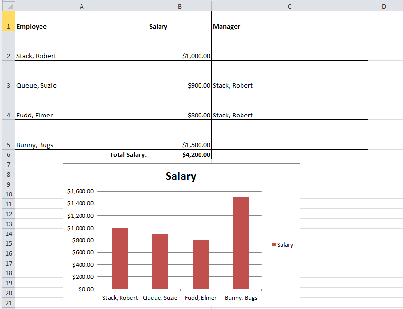
*** Note: The name tag page has an example about how to use Name tags to change named ranges' formulas dynamically with JETT formulas, indirectly updating a chart's data ranges.
Neither JETT nor Apache POI has an API to create a chart dynamically. However, both preserve features such as charts if found in the template spreadsheet. For charts to work in JETT, the chart must be created in the template spreadsheet. JETT won't actually do anything to the chart; it will only populate the data that the chart will use. Without the data in the template spreadsheet, certain steps must be taken to ensure proper display of the data in the chart in the resultant spreadsheet.
If the number of rows of data to display is known before transformation, then the chart can simply refer to the data cells that are known to be populated in the resultant spreadsheet.
In this example, it is known that there are 4 employees. The bar graph's data ranges are already entered. The x-axis values are $A$2:$A$5, and the only series is $B$2:$B$5. The "fixed" flag is set to true on the forEach tag, so that no shifting will occur for anything below the data.

...which gets transformed into...

It is possible to use charts even when the number of rows of data is not known beforehand. Normally, chart ranges are hard-coded into the template spreadsheet with a formula such as "Sheet1!$B$2:$B$5". But with the Excel formulas "OFFSET" and "COUNTA", and the Excel "defined names" feature, it is possible for chart range formulas to refer to a dynamic range of data. For Excel 2007+, look in the "Formulas" toolbar, then choose "Define Name". Enter any name, e.g. "DataLabels", plus the formula.
=OFFSET(Sheet1!$B$2, 0, 0, COUNTA(Sheet1!$B$2:$B$40), 1)
The Excel OFFSET formula produces a range of cells, whose top-left cell is the first cell argument. The range is translated by the next two arguments, which are the number of rows and columns. The range height and width are the next two columns. Here, the height is specified by a formula, resulting from the count of the values, and the width is one. Note that here, the values should not go beyond row 40 -- the "COUNTA" formula cuts off the data there. Then, the chart data simply refers to the defined name: "=Sheet1!DataLabels".